Gaussian Mixture Model
Recently, I started to learn some basic concepts and implementations about the famous "Gaussian Mixture Model". In this post, I'd like to share some key notes about this technique.
1. Clustering
Let's start with the problem of
clustering.
Goal: represent a data set in terms of K clusters each of which is summarized by a prototype \(\mu_{k}\).
One method to find these K cluster centers is to use the K-means technique.
In general, there are three major steps in its simplest version:
- Initialize prototypes (cluster centers): random select K cluster centers.
- Assign each data point to its nearest prototype.
- Update prototypes to be the cluster means.
Repeat step 2 and 3 until the algorithm converges (when the cluster centers are no longer changed).
Note that the simplest version is based on Euclidean distance.
Figure 1. K-means clustering. (from http://simplystatistics.org/)
To easily understand the general idea of clustering, consider the case that we have a dataset \(D=\{x_{1},x_{2},\cdots x_{n}\}\), each data \(x_i\) is a vector of length n, where n is the feature dimension. If n = 2, dataset D can be drawn in a 2D plane, each axis represents one of the two features (see Figure 1). For an unsupervised learning system, if we know there are totally 3 different kinds of data (3 class labels), then clustering can be used to classify the data point. The underlying assumption is: data belonging to the same class are supposed to have similar patterns so that they are more closer to each other. While data from different classes may have different patterns and their distance is far. So clustering is trying to find the class centers of each class, the more closer the data point lies in, the higher probability it has belonging to this class.
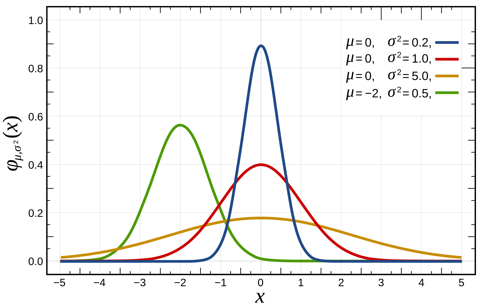
2. Gaussian Distribution
Gaussian Distribution in its 1-dimension form can be written as:
\[f(x, \mu, \sigma) = \dfrac{1}{\sigma\sqrt{2\pi}}e^{-\dfrac{(x-\mu)^2}{2\sigma^2}}\]
where, \(x\) is the data point, \(\mu\) is the mean of the data, and \(\sigma\) is the covariance.
In its 2D case:
\[f(x,\mu,\Sigma)=\dfrac{1}{(2\pi)^{d/2}\sqrt{|\Sigma|}}exp(-\dfrac{1}{2}(x-\mu)^{T}\Sigma^{-1}(x-\mu))\]
where, \(\Sigma\) is now the covariance matrix of the Gaussian.
Intuitively, \(\mu\) controls the "center position" of the Gaussian, \(\Sigma\) controls the "shape" the Gaussian.
Figure 2. Gaussian distribution (from en.wikipedia.org)
In many cases, when we want to model the random data (or more formally random variables), Gaussian distribution is very commonly used. Other common distributions are Bernoulli (p), Discrete Uniform, or Poisson distributions.
3. Maximum likelihood Estimation
Given a dataset \(X=\{x_{n}\}, n=1..N\), draw from an unknown distribution, assume the data follow a single Gaussian distribution, we can model the data using a Gaussian function.
Assume observed data points generated independently, the likelihood probability of the data can be written as:
\[p(X|\mu,\Sigma)=\Pi_{n=1}^{N}p(x_{n}|\mu,\Sigma)\], where \(p(x|\mu,\Sigma)\) is Gaussian distribution. This is called likelihood function.
The goal is to find parameters \(\mu\) and \(\Sigma\), of which the Gaussian distribution fits the data. In other words, the Gaussian is
most likely to be the "true" distribution of the data.
One of the solution of this problem, it called Maximum likelihood \(p(D|\mu,\Sigma)\). This can be also viewed as an optimization problem that:
\[\theta^{*}=\arg\max_{\theta}p(D|\theta)=\arg\max_{\theta}\Pi_{i=1}^{N}p(x_{i}|\theta)\]
,where \(\theta=\{\mu,\Sigma\}\)
To solve the optimization problem, there are many approaches. E.g.,
- Maximize the log likelihood. Take the "log" of the likelihood function, compute the derivative, set the gradient to zero, solve the equation to get the value of parameters.
- Expectation-Maximization (EM) approach. General idea of this approach lies in two steps, specifically:
- E-Step: Estimate the distribution of the hidden variable given the data and the current value of the parameters.
- M-Step: Maximize the joint distribution of the data and the hidden variable.
In this post, we will not cover all the math part of the approach. But intuitively, we can consider this approach like: Step 1, compute some measurement of the data using current parameters. Step 2, maximize the measurement by updating the parameters. Repeat doing these two steps, until the approach convergence. More details see the next section.
4. Gaussian Mixture Model
In order to model more complex data distribution, instead of using one Gaussian function, the linear combination of several Gaussian functions can be used. This is the basic concept of the Gaussian Mixture Model (GMM). Specifically,
\[p(x)=\Sigma_{k=1}^{K}\pi_{k}\mathcal{N}(X|\mu_{k},\Sigma_{k})\]
where \(\forall k:\pi_{k}\geq0,\Sigma_{k=1}^{K}\pi_{k}=1\)
Recall the definition of Gaussian, for a D-dimensional feature vector, \(x\), the mixture component \(p_i\), has a parameter of Dx1 mean vector and a DxD covariance matrix:
\[p_{i}(x)=\dfrac{1}{(2\pi)^{D/2}|\Sigma_{i}|^{1\2}}exp\left\{ -\dfrac{1}{2}(x-\mu_{i})'(\Sigma_{i})^{-1}(x-\mu_{i})\right\} \]
Fitting the Gaussian Mixture model is to get the parameters: \(\lambda=\{\omega_{i},\mu_{i},\Sigma_{i}\}\). We wish to model the data using the GMM, which means given the dataset, find the corresponding parameters :
- Mixing paramteres \(\pi\)
- Means \(\mu\)
- Covariances \(\Sigma\)
Figure 3 Gaussian Mixture Model
One of the method to fit the GMM to the data is the EM method. The EM algorithm iteratively refines the GMM parameters to increase the likelihood of the estimated model.
The hidden variable introduced in EM method for GMM is the "labels" (which component generate each data point). In other words, if we know for each point, which Gaussian generate it, by maximizing the likelihood of the data would results in the model parameters.
So the E-step of the EM: for each point, estimate the probability that each Gaussian generated it.
The M-step of the EM: modify the parameters according to the hidden variable to maximize the likelihood of the data (and the hidden variable).
5. Code & Example
In this section, we use the python library(module)
scikit learn to show how to use GMM.
First of all, import the related python module:
import numpy as np
from sklearn import mixture
import matplotlib.pyplot as plt
Then generate some random data for demo:
#Generate data
def gendata():
    obs = np.concatenate((1.6*np.random.randn(300, 2), 6 + 1.3*np.random.randn(300, 2), np.array([-5, 5]) + 1.3*np.random.randn(200, 2), np.array([2, 7]) + 1.1*np.random.randn(200, 2)))
    return obs
Also define the 2D Gaussian function for plotting:
def gaussian_2d(x, y, x0, y0, xsig, ysig):
    return 1/(2*np.pi*xsig*ysig) * np.exp(-0.5*(((x-x0) / xsig)**2 + ((y-y0) / ysig)**2))
To generate the GMM model:
#Generate GMM model and fit the data
def gengmm(nc=4, n_iter = 2):
    g = mixture.GMM(n_components=nc)  # number of components
    g.init_params = ""  # No initialization
    g.n_iter = n_iter   # iteration of EM method
    return g
To fit the GMM to the data, just call the .fit method, which will return the GMM with related parameters.
To plot the GMM model:
def plotGMM(g, n, pt):
    delta = 0.025
    x = np.arange(-10, 10, delta)
    y = np.arange(-6, 12, delta)
    X, Y = np.meshgrid(x, y)

    if pt == 1:
        for i in xrange(n):
            Z1 = gaussian_2d(X, Y, g.means_[i, 0], g.means_[i, 1], g.covars_[i, 0], g.covars_[i, 1])
            plt.contour(X, Y, Z1, linewidths=0.5)

    #print g.means_
    plt.plot(g.means_[0][0],g.means_[0][1], '+', markersize=13, mew=3)
    plt.plot(g.means_[1][0],g.means_[1][1], '+', markersize=13, mew=3)
    plt.plot(g.means_[2][0],g.means_[2][1], '+', markersize=13, mew=3)
    plt.plot(g.means_[3][0],g.means_[3][1], '+', markersize=13, mew=3)

    #plot the GMM with mixing parameters (weights)
    #i=0
    #Z2= g.weights_[i]*gaussian_2d(X, Y, g.means_[i, 0], g.means_[i, 1], g.covars_[i, 0], g.covars_[i, 1])
    #for i in xrange(1,n):
    #    Z2 = Z2+ g.weights_[i]*gaussian_2d(X, Y, g.means_[i, 0], g.means_[i, 1], g.covars_[i, 0], g.covars_[i, 1])
    #plt.contour(X, Y, Z2)
The main function:
obs = gendata()
fig = plt.figure(1)
g = gengmm(4, 100)
g.fit(obs)
plt.plot(obs[:, 0], obs[:, 1], '.', markersize=3)
plotGMM(g, 4, 0)
plt.title('Gaussian Mixture Model')
plt.show()
To intuitively show how EM approach works, Gaussian mixtures fitted in different iterations can be plotted:
g = gengmm(4, 1)
g.fit(obs)
plt.plot(obs[:, 0], obs[:, 1], '.', markersize=3)
plotGMM(g, 4, 1)
plt.title('Gaussian Models (Iter = 1)')
plt.show()

g = gengmm(4, 5)
g.fit(obs)
plt.plot(obs[:, 0], obs[:, 1], '.', markersize=3)
plotGMM(g, 4, 1)
plt.title('Gaussian Models (Iter = 5)')
plt.show()

g = gengmm(4, 20)
g.fit(obs)
plt.plot(obs[:, 0], obs[:, 1], '.', markersize=3)
plotGMM(g, 4, 1)
plt.title('Gaussian Models (Iter = 20)')
plt.show()

g = gengmm(4, 100)
g.fit(obs)
plt.plot(obs[:, 0], obs[:, 1], '.', markersize=3)
plotGMM(g, 4, 1)
plt.title('Gaussian Models (Iter = 100)')
plt.show()
The plot of different iterations in EM method shows in the following, one can see that the Gaussian models are incrementally updated and refined to fit the data. Both the means (cross markers in the figure) and covariances (curves in the figures) are updated during the iteration, until the approach converges.
Figure 4 Gaussian Mixture Model fitted using different EM iterations.
If we consider the GMM with the weights (Mixing parameters \(\pi\)), the plotting is shown like the following figure:
Figure 5 Gaussian Mixture Model after iterations of EM approach (draw with weights)